1671年、スコットランドのジェームス・グレゴリーが発見した $~\tan^{-1}x~$ に関する級数です。この級数によって、円周率の近似値の研究が格段に進みました。グレゴリー級数の値の算出から、円周率の近似の方法について紹介します。
①グレゴリー級数
②証明
③$ \displaystyle x=1 $のとき(ライプニッツ級数)
④$ x=\frac{1}{\sqrt{3}} $のとき(シャープの計算)
⑤$ \displaystyle x=\sqrt{3} $のとき(おまけ)
※このサイトでは、ライプニッツ級数を一般化したものをグレゴリー級数としていますが、まとめて「グレゴリー・ライプニッツ級数」と呼んだり、諸説あるようです。
①グレゴリー級数
グレゴリー級数は、1671年にスコットランドのジェームス・グレゴリーが発見した級数であり、その後の円周率の近似で大変重要な役割を果たしました。まずは、グレゴリー級数とはどのようなものかを見てみましょう。
次のような級数をグレゴリー級数という。
\begin{equation}
\displaystyle \tan^{-1}x=\sum_{n=0}^{\infty}\frac{(-1)^n}{2n+1}x^{2n+1}
\end{equation}
右辺が $~\sum~$ 記号でわかりにくいので、見やすくすると・・
\begin{equation}
\displaystyle x-\frac{1}{3}x^3+\frac{1}{5}x^5-\frac{1}{7}x^7+\cdots
\end{equation}
となります。
以前の紹介したライプニッツ級数と形が非常に似ていますね。
実は、グレゴリー級数に $~x=1~$ を代入すると、ライプニッツ級数になります。そのため、「グレゴリー・ライプニッツ級数」と呼ばれることもあります。(詳しくは③$ \displaystyle x=1 $のとき(ライプニッツ級数)へ)
②証明
ライプニッツ級数とほぼ同じ流れで証明をすることができます。
初項 $~1~$ 、公比 $~-t^2(0 \le t <1)~$ の無限等比級数を考えると、|公比|$<1~$ より、次のような関係式が表せる。
\begin{equation}
\displaystyle 1-t^2+t^4-t^6+\cdots=\frac{1}{1-(-t^2)}=\frac{1}{1+t^2}
\end{equation}
ここで、 $~t:0 \to x~$ について、両辺積分をとると、
\begin{equation}
\displaystyle \int_{0}^{x}( 1-t^2+t^4-t^6+\cdots)dt=\int_{0}^{x}\frac{1}{1+t^2}dt ・・(*)
\end{equation}
であり、左辺と右辺それぞれを計算する。左辺について計算していくと、
\begin{align}
\displaystyle (左辺)&=\int_{0}^{x}( 1-t^2+t^4-t^6+\cdots)dt \\
\\
&=\left[ t-\frac{1}{3}t^3+\frac{1}{5}t^5-\frac{1}{7}t^7+\cdots \right]_{0}^{x} \\
\\
&=x-\frac{1}{3}x^3+\frac{1}{5}x^5-\frac{1}{7}x^7+\cdots
\end{align}
となる。右辺に関しては、 $~t=\tan{\theta}~$ と置換することで、
$~ t:0 \to x ~$ が $~\theta :0 \to \tan^{-1}x ~$ となり、 $~ \displaystyle dt=\frac{1}{\cos^{2} \theta}d \theta ~$ となるため、
\begin{align}
\displaystyle (右辺)&=\int_{0}^{x}\frac{1}{1+t^2}dt \\
\\
&=\int_{0}^{\tan^{-1}x}\frac{1}{1+\tan^{2}\theta}\cdot \frac{1}{\cos^{2} \theta}d \theta \\
\\
&=\int_{0}^{\tan^{-1}x} \cos^{2}\theta \cdot \frac{1}{\cos^{2} \theta}d \theta \\
\\
&=\int_{0}^{\tan^{-1}x}d \theta \\
\\
&=[\theta]_{0}^{\tan^{-1}x} \\
\\
&=\tan^{-1}x
\end{align}
と右辺も求まった。
左辺と右辺の計算結果を元の等式$(*)$に代入することで、
\begin{equation}
\displaystyle x-\frac{1}{3}x^3+\frac{1}{5}x^5-\frac{1}{7}x^7+\cdots=\tan^{-1}x
\end{equation}
となり、グレゴリー級数が示された。 $~\blacksquare$
初項 $~1~$ 、公比 $~-t^2(0 \le t <1)~$ の無限等比級数を考えると、|公比|$<1~$ より、次のような関係式が表せる。
\begin{align}
&\displaystyle 1-t^2+t^4-t^6+\cdots \\
\\
&=\frac{1}{1-(-t^2)} \\
\\
&=\frac{1}{1+t^2}
\end{align}
ここで、 $~t:0 \to x~$ について、両辺積分をとると、
\begin{equation}
\displaystyle \int_{0}^{x}( 1-t^2+t^4-\cdots)dt=\int_{0}^{x}\frac{1}{1+t^2}dt
\end{equation}
である。・・・・(*)
(*)の左辺と右辺それぞれを計算する。
左辺について計算していくと、
\begin{align}
\displaystyle (左辺)&=\int_{0}^{x}( 1-t^2+t^4-t^6+\cdots)dt \\
\\
&=\left[ t-\frac{1}{3}t^3+\frac{1}{5}t^5-\frac{1}{7}t^7+\cdots \right]_{0}^{x} \\
\\
&=x-\frac{1}{3}x+\frac{1}{5}x-\frac{1}{7}x+\cdots
\end{align}
となる。右辺に関しては、 $~t=\tan{\theta}~$ と置換することで、
$~ t:0 \to x ~$ が $~\theta :0 \to \tan^{-1}x ~$ となり、 $~ \displaystyle dt=\frac{1}{\cos^{2} \theta}d \theta ~$ となるため、
\begin{align}
\displaystyle (右辺)&=\int_{0}^{x}\frac{1}{1+t^2}dt \\
\\
&=\int_{0}^{\tan^{-1}x}\frac{1}{1+\tan^{2}\theta}\cdot \frac{1}{\cos^{2} \theta}d \theta \\
\\
&=\int_{0}^{\tan^{-1}x} \cos^{2}\theta \cdot \frac{1}{\cos^{2} \theta}d \theta \\
\\
&=\int_{0}^{\tan^{-1}x}d \theta \\
\\
&=[\theta]_{0}^{\tan^{-1}x} \\
\\
&=\tan^{-1}x
\end{align}
と右辺も求まった。
左辺と右辺の計算結果を元の等式$(*)$に代入することで、
\begin{equation}
\displaystyle x-\frac{1}{3}x+\frac{1}{5}x-\frac{1}{7}x+\cdots=\tan^{-1}x
\end{equation}
となり、グレゴリー級数が示された。 $~\blacksquare$
逆三角関数を使って一般化しているため、証明の難易度はライプニッツ級数より上がります・・。
③$ \displaystyle x=1 $のとき(ライプニッツ級数)
グレゴリー級数の $~x~$ に、ある値を代入することで円周率の近似計算を行うことができます。例えば、 $~x=1~$ を代入すると、
\begin{align}
(左辺)&=\tan^{-1}1 \\
&=\displaystyle \frac{\pi}{4}\\
\\
(右辺)&=1-\frac{1}{3}+\frac{1}{5}-\frac{1}{7}+\cdots
\end{align}
となり、まとめると先ほどから登場しているライプニッツ級数となります。
次のような級数をライプニッツ級数という。
\begin{align}
\displaystyle \frac{\pi}{4}&=\sum_{n=0}^{\infty}\frac{(-1)^n}{2n+1} \\
\\
&=1-\frac{1}{3}+\frac{1}{5}-\frac{1}{7}+\cdots
\end{align}
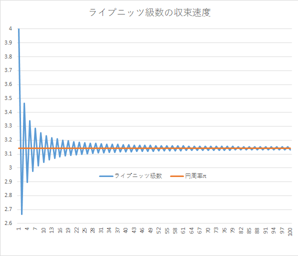
この式を使って、計算する右辺の項を増やしながら円周率を算出すると、次のように円周率の値が近似されていきます。
| 計算した右辺の項の数 | 円周率の近似値 |
|---|---|
| 1$\left(\displaystyle \frac{\pi}{4}=1\right) $ | 4 |
| 2$ \left(\displaystyle \frac{\pi}{4}=1-\frac{1}{3}\right)$ | 2.66666666 |
| 3$ \left(\displaystyle \frac{\pi}{4}=1-\frac{1}{3}+\frac{1}{5}\right)$ | 3.46666666 |
| 4$ \left(\displaystyle -\frac{1}{7} \text{の項まで} \right)$ | 2.89523809 |
| 5$ \left(\displaystyle +\frac{1}{9} \text{の項まで} \right)$ | 3.33968254 |
| \begin{equation}\vdots \end{equation} | \begin{equation}\vdots \end{equation} |
| 10$ \left(\displaystyle -\frac{1}{19} \text{の項まで} \right)$ | 3.04183961 |
| \begin{equation}\vdots \end{equation} | \begin{equation}\vdots \end{equation} |
| 100$ \left(\displaystyle -\frac{1}{199} \text{の項まで} \right)$ | 3.13159290 |
実際の円周率の値への近づき方をグラフにすると、次のようになります。
④$ x=\frac{1}{\sqrt{3}} $のとき(シャープの計算)
グレゴリー級数から円周率を近似するには、 $~x=1~$ 以外でもできます。$ \displaystyle x=\frac{1}{\sqrt{3}} $を代入してみましょう。
\begin{align}
\displaystyle(左辺)&=\tan^{-1}\frac{1}{\sqrt{3}} \\
&=\displaystyle \frac{\pi}{6} \\
\\
(右辺)&=\frac{1}{\sqrt{3}}-\frac{1}{3}\cdot \frac{1}{3\sqrt{3}} +\frac{1}{5}\cdot \frac{1}{9\sqrt{3}}-\cdots \\
\\
&=\frac{\sqrt{3}}{3} \left( 1-\frac{1}{3}\cdot \frac{1}{3}+\frac{1}{5}\cdot \frac{1}{9}-\cdots \right)
\end{align}
となり、円周率を求めることができそうです。
実際、1699年にイギリス人のエイブラハム・シャープがこの式で小数第72位まで円周率を計算しました。さらに、1719年にはフランスのトーマス・ラグニーが同様の式で小数第127位まで円周率を計算しています。
先ほどと同様に右辺の項の数を順々に増やして、円周率の近似値を求めていきます。
| 計算した右辺の項の数 | 円周率の近似値 |
|---|---|
| 1$\left(\displaystyle \frac{\pi}{6}=\frac{\sqrt{3}}{3}\left( 1 \right) \right) $ | 3.46410161 |
| 2$ \left(\displaystyle \frac{\pi}{6}=\frac{\sqrt{3}}{3}\left( 1-\frac{1}{3}\cdot \frac{1}{3} \right) \right) $ | 3.07920143 |
| 3$ \left(\displaystyle \frac{\pi}{6}=\frac{\sqrt{3}}{3}\left( 1-\frac{1}{3}\cdot \frac{1}{3}+\frac{1}{5}\cdot \frac{1}{9} \right) \right) $ | 3.15618147 |
| 4$ \left(\displaystyle -\frac{1}{7}\cdot \frac{1}{27} \text{の項まで} \right)$ | 3.13785289 |
| 5$ \left(\displaystyle +\frac{1}{9}\cdot \frac{1}{81} \text{の項まで} \right)$ | 3.14260474 |
| \begin{equation}\vdots \end{equation} | \begin{equation}\vdots \end{equation} |
| 10$ \left(\displaystyle -\frac{1}{19}\cdot \frac{1}{3^9} \text{の項まで} \right)$ | 3.14159051 |
| \begin{equation}\vdots \end{equation} | \begin{equation}\vdots \end{equation} |
| 100$ \left(\displaystyle -\frac{1}{199}\cdot \frac{1}{3^{99}} \text{の項まで} \right)$ | 3.14159265 |
100項目まで計算すると、エクセルでは誤差が表れないほど正確になってきました。グラフにすると、次のようになります。
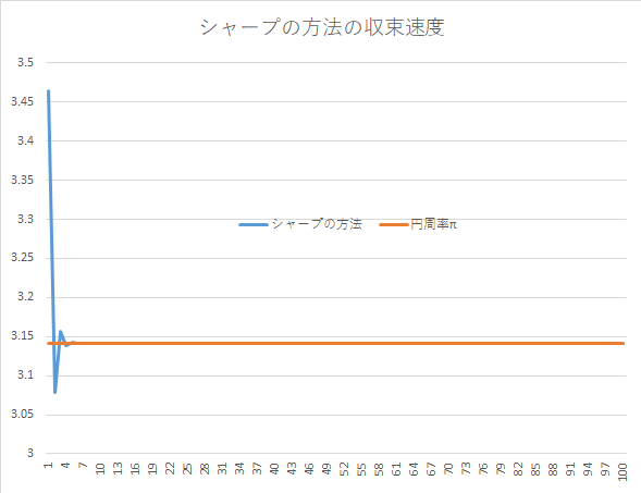
ライプニッツ級数やウォリスの公式に比べ、収束速度が非常に速いことがわかります。すなわち、少ない計算でより細かいケタまで、円周率が計算できるということです。
⑤$ \displaystyle x=\sqrt{3} $のとき(おまけ)
今まで $~\tan^{-1}x~$ の値がわかりやすくなるように、 $~x~$ の値を決めて計算してきました。では、グレゴリー級数に$ \displaystyle x=\sqrt{3} $を代入したらどうなるのでしょうか?
実は、級数が収束しないため、値が求まりません。
グレゴリー級数の右辺に$ x=\sqrt{3} $を代入すると、
\begin{align}
(右辺)\displaystyle &=\sum_{n=0}^{\infty}\frac{(-1)^n}{2n+1}\sqrt{3}^{2n+1}
\end{align}
となります。ここで、ダランベールの収束判定法を使うと、
\begin{align}
\displaystyle \left| \frac{a_{n+1}}{a_{n}} \right|&=\left| \frac{\frac{(-1)^{n+1}}{2n+3}\sqrt{3}^{2n+3}}{\frac{(-1)^n}{2n+1}\sqrt{3}^{2n+1}} \right|\\
\\
&=\left| (-1)\cdot \frac{2n+1}{2n+3}\cdot 3 \right| \\
\\
&=\left| (-1)\cdot \frac{6n+3}{2n+3} \right| \\
\\
&>1
\end{align}
であるため、この場合のグレゴリー級数は発散します。注意してください。
ライプニッツ級数の一般化させたグレゴリー級数の話でした。それにしてもシャープの方法は収束速度が速いですね・・・。

☆参考文献等
・「Wikipedia 円周率の歴史」,<https://ja.wikipedia.org/wiki/%E5%86%86%E5%91%A8%E7%8E%87%E3%81%AE%E6%AD%B4%E5%8F%B2 > 2017年3月24日アクセス
・「Wikipedia ジェームス・グレゴリー」,<https://ja.wikipedia.org/wiki/%E3%82%B8%E3%82%A7%E3%83%BC%E3%83%A0%E3%82%B9%E3%83%BB%E3%82%B0%E3%83%AC%E3%82%B4%E3%83%AA%E3%83%BC > 2017年3月24日アクセス
コメント
コメント一覧 (2件)
グレゴリー級数の証明のとこ
積分後の級数のxの指数が抜けてます
コメントありがとうございます。
修正いたしました!!